Get Your Custom Quote

Online Inquiry

Deep Proteome Profiling — 8,000–12,000+ Protein Groups for Biomarker Discovery, Target Identification & Multi-Omics Integration

Go beyond the 3,000–5,000 protein ceiling of standard shotgun proteomics. Our multi-dimensional fractionation combined with DIA/4D-DIA/TMT on latest-generation MS platforms captures the low-abundance regulatory proteins — kinases, transcription factors, receptors, signalling nodes — that standard workflows systematically miss.

Research Use Only (RUO) Notice: All services and data provided are strictly for non-clinical research purposes. Our analytical results are not intended for clinical diagnosis, patient management, or therapeutic decision-making.

Services Technologies Demo Case Study FAQ Related Services

CORE SERVICE

Coverage Depth That Changes What You Can Discover

The number of proteins you can detect determines the biological questions you can answer. A standard shotgun proteomics experiment — single-shot DDA or DIA without fractionation — routinely identifies 3,000–5,000 protein groups from a cell or tissue lysate. That is enough to catalogue abundant enzymes and structural proteins, but it systematically excludes the low-copy-number regulators — kinases, transcription factors, E3 ubiquitin ligases, membrane receptors, and signalling adaptors — that control phenotype, drive disease, and constitute the most valuable drug targets and biomarkers.

Our Deep Proteome Profiling service is purpose-built for researchers who have hit this coverage ceiling. By adding one or two orthogonal fractionation dimensions before LC-MS/MS analysis — peptide-level high-pH RP or HILIC fractionation, optionally combined with protein-level SEC or SDS-PAGE — we routinely deliver 8,000–12,000+ protein groups per sample. This 2–3× depth gain is the difference between seeing the housekeeping proteome and seeing the regulatory proteome.

  • For biomarker discovery teams: Detect tissue-derived, low-abundance proteins in plasma — not just acute-phase reactants — and expand your candidate pool 3–5×
  • For drug target discovery: Capture kinases, transcription factors, and membrane proteins at 10–1,000 copies/cell that single-shot workflows miss
  • For multi-omics studies: Achieve >50% proteome-to-transcriptome mapping coverage, enabling meaningful cross-omics correlation
Deep proteome profiling workflow showing multi-dimensional fractionation and LC-MS/MS analysis pipeline

Figure 1. Deep proteome profiling workflow: multi-dimensional fractionation → LC-MS/MS acquisition → 10,000+ protein group identification.

Biomarker Discovery Needs Depth — Low-Abundance Proteins Carry the Tissue-Specific Signal

The classical biomarker discovery paradigm holds that the most informative biomarkers are often the least abundant proteins: tissue-specific secreted proteins, shed receptor ectodomains, or signalling molecules that change concentration before abundant housekeeping proteins do. Yet standard plasma proteomics — even with high-abundance protein depletion — routinely identifies fewer than 500–800 proteins, dominated by albumin, immunoglobulins, and acute-phase reactants. Most tissue-derived candidate biomarkers are present in plasma at ng/mL concentrations or below, well below the detection limit of single-shot workflows.

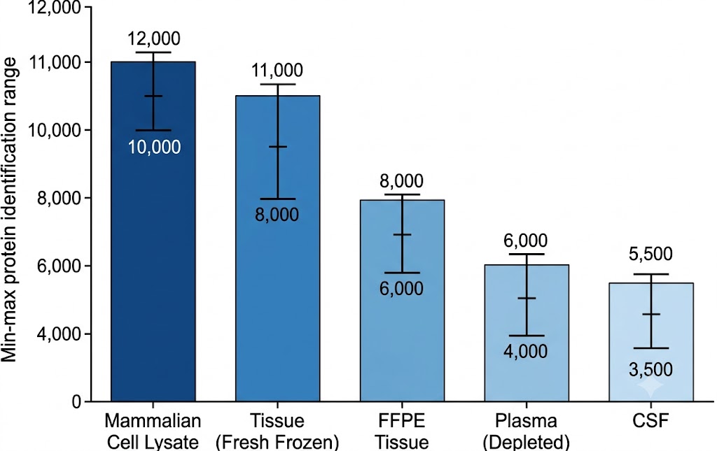
Deep Proteome Profiling addresses this through a combination of abundant protein depletion (where applicable), peptide-level fractionation, and DIA acquisition that together expand the detectable plasma proteome to 4,000–6,000 proteins. At this depth, tissue-specific proteins — brain-derived, cardiac, liver-secreted, tumour-associated — become detectable in the circulation. In published cohort studies using similar workflows, this depth expansion has directly translated to the identification of candidate biomarkers that were invisible to standard plasma proteomics, including proteins involved in neuronal signalling, extracellular matrix remodelling, and immune regulation — the very categories most likely to carry disease-specific information.

Drug Target Discovery Requires Access to the Regulatory Proteome

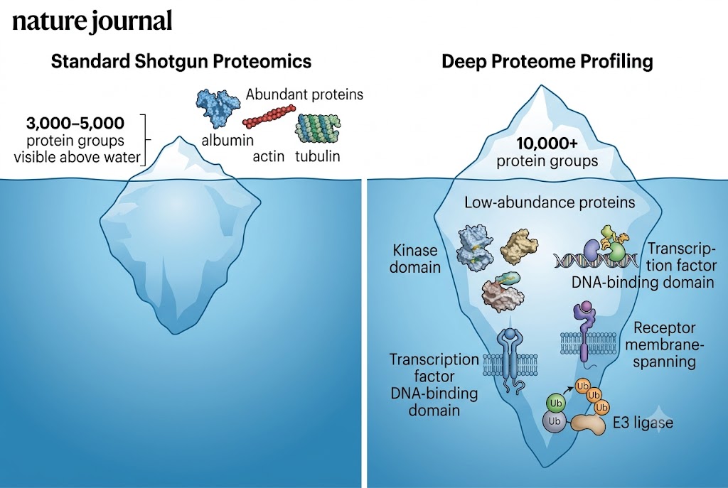
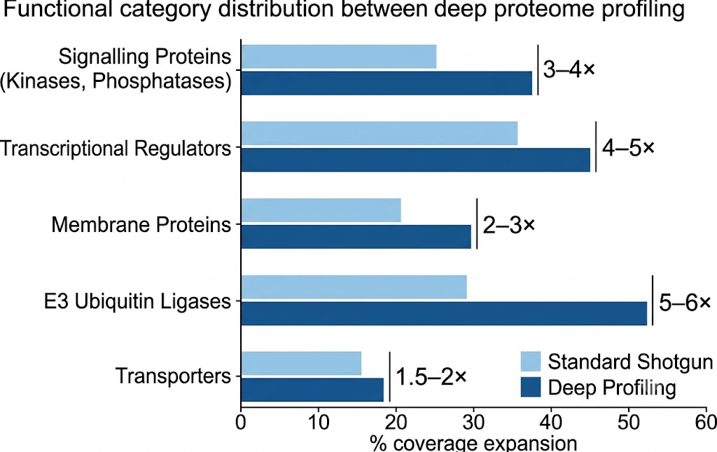
If your research question is mechanistic rather than descriptive — you want to know which signalling pathways are activated, which transcription factors drive the response, or which ubiquitin ligases regulate a substrate — then coverage of low-abundance proteins is not a luxury; it is a prerequisite. Kinase cascades, ubiquitin signalling networks, transcriptional regulation complexes, and protein-protein interaction modules are all executed by proteins expressed at copy numbers too low for single-shot shotgun proteomics to detect.

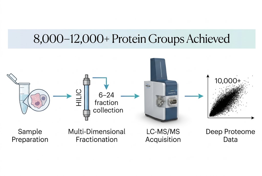
With deep profiling, we routinely identify 200–400 protein kinases and 50–150 transcription factors from a mammalian cell lysate — the difference between seeing the downstream readout (a phosphorylated protein) and seeing the upstream kinase that phosphorylated it. This depth enables target discovery scientists to map signalling networks from input to effector, not just from effector to phenotype.

Multi-Omics Integration Depends on Proteome Completeness

A common frustration in multi-omics studies is the asymmetry between transcriptome coverage (15,000–20,000 detected transcripts by RNA-seq) and proteome coverage (3,000–5,000 proteins by standard shotgun MS). This gap means that for every five genes that change at the RNA level, you have proteomics data for only one — making correlation analysis statistically unreliable and pathway-level interpretation heavily biased toward abundant proteins.

Deep Profiling closes this gap. At 10,000+ protein groups, the proteome-to-transcriptome mapping fraction rises to >50%, enabling meaningful correlation analysis across omics layers. Differentially expressed transcripts can be checked for corresponding protein-level changes; pathway enrichment can be computed on both omics layers with comparable coverage; and the integration analysis shifts from "what can we detect" to "what is biologically consistent."

Comparison of proteome coverage: standard shotgun vs deep profiling across sample types

How We Achieve 8,000–12,000+ Protein Groups: Fractionation, Acquisition & Quantification Strategies

Multi-Dimensional Peptide Fractionation

The primary driver of depth is pre-MS fractionation. We deploy high-pH reversed-phase fractionation (HPRP) and hydrophilic interaction liquid chromatography (HILIC) as the first dimension, each separating the peptide mixture into 6–24 orthogonal fractions before conventional low-pH RP-LC-MS/MS analysis. Each fraction contains fewer co-eluting peptides, reducing ion suppression and enabling MS detection of low-abundance species that would be masked in a single-shot run. The fractionation depth is adjustable: fewer fractions (6–8) for moderate depth gain with lower cost; more fractions (12–24) when maximum coverage is the priority.

DIA & 4D-DIA Acquisition

Data-independent acquisition (DIA) systematically fragments all precursors within defined isolation windows, producing complete fragment ion maps. Unlike data-dependent acquisition (DDA), which selects only the most abundant precursors for fragmentation, DIA captures fragment data for every detectable precursor — including low-abundance ions that trigger MS/MS only sporadically in DDA mode. On the Bruker timsTOF Pro platform, 4D-DIA adds ion mobility separation (TIMS) as a fourth dimension, further reducing spectral complexity and improving detection of co-eluting low-abundance peptides by 15–30% over 3D-DIA alone.

TMT Multiplexing for Multi-Condition Comparisons

When the study involves comparing multiple conditions, time points, or treatment groups, TMT (tandem mass tag) 16-plex labelling enables all samples in a multiplex set to be combined, fractionated, and analysed together in a single workflow. This eliminates the fractionation throughput bottleneck — one fractionation set serves all 16 samples simultaneously — and removes between-run fractionation variability as a source of technical noise. TMT-based deep profiling is the method of choice for time-course studies, dose-response experiments, and any multi-group comparison where inter-sample normalisation is critical.

Standardized Workflow

1. Sample preparation and protein extraction: Proteins are extracted using the optimal method for the sample type (RIPA for tissue, SDC-SPE for plasma, Trizol for cells). Concentration measured by BCA assay.

2. Digestion and peptide cleanup: Reduction (DTT/TCEP), alkylation (IAA), trypsin digestion (or alternative protease). Desalting and concentration by C18 SPE.

3. Multi-dimensional fractionation: Peptides separated by high-pH RP or HILIC into 6–24 fractions. For TMT: all labels combined before fractionation.

4. LC-MS/MS acquisition: Each fraction analysed on timsTOF Pro (4D-DIA), Exploris 480 (DIA), or Orbitrap Astral-class. QC standards at regular intervals.

5. Database search and quantification: Spectronaut, DIA-NN, or Proteome Discoverer pipeline. FDR ≤1% at peptide and protein levels. Normalised protein group output with CV and missing-value statistics.

6. Bioinformatics and reporting: Differential expression analysis, pathway enrichment (GO, KEGG, Reactome), protein interaction networks, multi-omics integration support. Comprehensive report with methods, results tables, and visualisations.

Sample Requirements for Deep Proteome Profiling

Sample Type Recommended Input Minimum Input Special Considerations
Cell lysate (adherent / suspension / primary) 200 µg protein 10 µg ≥1 × 10⁶ cells for standard input; low-input workflows available for rare populations
Tissue (fresh frozen) 5–20 mg wet weight 1–2 mg Homogenisation method optimisable per tissue type; laser-capture microdissection compatible
FFPE tissue 2–10 sections (10 µm thickness) 1 section (10 µm) Deparaffinisation and heat-induced antigen retrieval required; protein yield variable by tissue and fixation time
Plasma / Serum 50–100 µL 10 µL High-abundance protein depletion (MARS-14 or ProteoMiner) strongly recommended; EDTA plasma preferred over heparin
CSF 100–200 µL 50 µL Low protein concentration (0.15–0.45 mg/mL typical); minimal volume acceptable with reduced depth
Exosomes / Extracellular vesicles 100 µg protein equivalent 25 µg Isolation method (SEC, UC, precipitation) should be specified for data interpretation
Saliva / Urine / Other biofluids 1–5 mL 500 µL Variable protein concentration; precipitation or lyophilisation recommended before digestion
Subcellular fractions (nuclear / cytoplasmic / membrane / mitochondrial) 100 µg protein 25 µg Fraction purity should be validated (western blot or enzyme assay) before MS analysis

Typical Deep Proteome Profiling Results: What You Can Expect

The figures below illustrate the types of results routinely obtained from deep profiling projects across diverse sample types. These representative outputs — protein group identification bar charts, quantitative reproducibility assessments, and functional annotation distributions — are examples of the standard deliverable format; your specific results will depend on sample type, input amount, and the biological system under study.

Protein group identification counts across sample types from deep proteome profiling

Figure 2. Typical protein group identification ranges by sample type. Cell/tissue lysates with 12-fraction HILIC + DIA routinely yield 8,000–12,000 protein groups; plasma/serum with depletion + 8-fraction HPRP yields 4,000–6,000; CSF and low-input samples yield proportionally fewer but with comparable reproducibility.

Quantitative reproducibility assessment showing CV distribution across technical and biological replicates

Figure 3. Quantitative reproducibility across biological replicates. DIA-based deep profiling workflows maintain median CV <15% with <5% missing values across replicates — essential for reliable differential expression analysis in cohort studies.

Functional annotation distribution of proteins identified by deep profiling vs standard shotgun

Figure 4. Functional category enrichment in deep profiling data compared to standard shotgun. Deep profiling preferentially expands coverage of signalling proteins (kinases, phosphatases), transcriptional regulators, and membrane proteins — the categories most relevant to drug target discovery and biomarker identification.

CASE STUDY

Hybrid DDA/DIA-PASEF Library Enables Deep Proteotyping of Triple-Negative Breast Cancer Tissues

Deep Profiling in TNBC Research

Background & Purpose

Triple-negative breast cancer (TNBC) is the most aggressive breast cancer subtype, characterised by high molecular heterogeneity and a lack of targeted therapies. Comprehensive proteomic characterisation of TNBC tissues is essential for understanding disease mechanisms and identifying new therapeutic targets. However, the depth and reproducibility of proteomic coverage across large TNBC cohorts had been limited by the absence of a dedicated spectral assay library optimised for TNBC tissue proteomes. This study aimed to construct a deep, TNBC-specific DDA/DIA-PASEF assay library and evaluate its quantitative performance against library-free approaches.

Methods

Total proteins were extracted from 105 TNBC tissue specimens and pooled. The pooled lysate was fractionated by HILIC chromatography into 12 fractions, each analysed by LC-MS/MS in DDA-PASEF mode on a Bruker timsTOF Pro mass spectrometer. A hybrid spectral library was generated using Spectronaut software. Sixteen individual TNBC tissue lysates were then analysed in DIA-PASEF mode and quantified using both the hybrid library (library-based) and direct DIA library-free approaches for comparison.

Results

The hybrid library contained 244,464 precursors, 168,006 peptides, and 11,564 protein groups at 1% FDR — the deepest TNBC proteome library reported to date. In the quantitative analysis of 16 individual tissues, library-based DIA quantification using Spectronaut achieved 190,310 precursors, 140,566 peptides, and 10,463 protein groups quantified per run, substantially outperforming library-free approaches on the same instrument platform.

Experimental workflow for DDA/DIA-PASEF hybrid library construction and DIA quantification

Figure 5. Experimental workflow: HILIC fractionation of pooled TNBC lysates → DDA-PASEF library construction → DIA-PASEF quantification of individual tissues.

Comparison of protein and precursor identifications between library-based and library-free DIA

Figure 6. Library-based DIA quantification achieved ~10,500 protein groups per individual tissue — substantially deeper than library-free DIA on the same instrument and samples.

Identification consistency across individual TNBC tissue samples

Figure 7. Protein identification consistency across 16 individual TNBC tissues, demonstrating the reproducibility of DIA-based deep profiling at cohort scale.

Why This Matters for Your Deep Profiling Project

This study demonstrates that deep fractionation (12-fraction HILIC) combined with DIA acquisition achieves approximately 10,500 protein groups from individual tissue samples — a depth that enables pathway-level biology, not just protein cataloguing. While this case focused on TNBC, the methodological framework — deep fractionation, hybrid library strategy, DIA quantification — is directly transferable to any tissue type, biofluid, or disease area. It represents the performance standard we deliver for Deep Proteome Profiling projects at Creative Proteomics.

Frequently Asked Questions

Q1: I have a limited sample amount — can I still get deep coverage?

Yes. Our sample input minimum is 10 µg of protein (approximately 1 × 10⁵–1 × 10⁶ cells depending on cell type). With input below 50 µg, we reduce the fractionation depth (4–6 fractions instead of 12–24) to match the available material. The coverage will be proportionally lower than with standard input, but still 2–3× deeper than single-shot analysis of the same sample. Please contact us for a feasibility assessment if your sample is below 10 µg.

Q2: How many kinases, transcription factors, or membrane proteins can I expect to detect?

From a mammalian cell lysate with 12-fraction deep profiling, we routinely detect 200–400 protein kinases (including most kinase families), 50–150 transcription factors, and 300–600 membrane proteins (depending on the enrichment efficiency). These numbers are 3–5× higher than single-shot shotgun proteomics from the same sample. The exact counts depend on cell type, expression levels, and input amount.

Q3: Can deep profiling handle cohort-scale studies with dozens or hundreds of samples?

Yes — but the experimental design differs from single-sample deep profiling. For cohort studies, we recommend TMT multiplexing (up to 16 samples per batch, all fractionated together) or label-free DIA with a standardised single-shot or limited-fraction workflow applied consistently across all samples. Full 12–24 fraction deep profiling of hundreds of individual samples is generally not cost-effective; instead, we design a fit-for-purpose workflow that balances depth with throughput. For maximum-depth studies on limited cohort sizes (≤50 samples), individual sample fractionation with DIA acquisition is the preferred approach.

Q4: How does the cost compare with standard proteomics, and when does deep profiling justify the premium?

Deep Profiling carries a higher per-sample cost than single-shot proteomics because each sample requires 6–24× more LC-MS/MS instrument time. However, when the research question depends on detecting low-abundance proteins — biomarker discovery, drug target identification, signalling network mapping — the per-protein cost is often comparable or lower, because the additional fractionation cost is small relative to the biological information gained. We recommend Deep Profiling when: (1) you need to detect proteins below the 5,000-protein ceiling, (2) your candidate list includes low-abundance categories (kinases, TFs, receptors), or (3) you need proteome coverage >50% of the transcriptome for multi-omics integration.

Q5: What bioinformatics support is included with the service?

Our standard deliverable includes: normalised protein-group-level expression matrix, differential expression analysis (volcano plots, PCA, heatmaps), GO/KEGG/Reactome pathway enrichment, and protein interaction network analysis. For multi-omics studies, we provide correlation matrices and integrated pathway enrichment. Custom bioinformatics (kinase enrichment analysis, transcription factor target enrichment, time-course clustering, machine learning classification) is available on request.

Q6: Can I use my own data analysis pipeline with the raw data?

Yes. We deliver raw MS data files (.d, .raw, or .wiff format depending on the instrument), search engine output files, and the normalised quantification matrix. All standard formats are compatible with downstream analysis platforms including Perseus, R/Bioconductor, and commercial tools. We can also export results in format-specific data tables for your preferred analysis pipeline.

References

  1. Lapcik P, Synkova K, Janacova L, Bouchalova P, Potesil D, Nenutil R, Bouchal P. A hybrid DDA/DIA-PASEF based assay library for a deep proteotyping of triple-negative breast cancer. Sci Data. 2024;11:794.
  2. Lou R, Liu W, Li R, Li S, He Q, Shui W. Acquisition and analysis of DIA-based proteomic data: a comprehensive survey in 2023. Mol Cell Proteomics. 2024;23(4):100713.
  3. Kawashima Y, Watanabe E, Umeyama T, Nakajima D, Hattori M, Honda K, Ohara O. Optimized data-independent acquisition approach for proteome coverage at the single-cell level. J Proteome Res. 2024;23(3):1028-1038.

GET STARTED

Push Past the Coverage Ceiling

Reach the proteins that matter most. Contact Creative Proteomics to design a Deep Proteome Profiling strategy matched to your research question, sample type, and budget.

Ready to go deeper?

Request a Customized Quote